

SITCOMTN-162
Testing the implementation of Metadetection and Cell-Based Coadds on Abell 360 LSSTComCam data#
Abstract
The purpose of this technote is to test the technical quality of LSSTComCam commissioning data, specifically the Rubin_SV_38_7 field, by utilizing cell-based coadds and Metadetection by measuring the tangential and cross weak lensing shear profiles of the massive cluster Abell 360 (called A360 throughout the technote). The process entails generating the cell-based coadds for Metadetection to run on, identifying and removing cluster member galaxies, applying quality cuts, calibrating the shear measurements, and validation.
Cell-based coadds and Metadetection are both currently in the process of being implemented within the LSST Science Pipelines at the time of this technote. There is substantial technical value in attempting a difficult measurement prior to full implementation. Measuring the tangential shear around A360 will showcase the current abilities of these algorithms, as well as highlight where work is still needed. As seen from the resulting shear profile of A360, the cell-based coadds and Metadetection are able to work in tandem to produce a shear catalog and resulting reduced shear profile.
This technote is one part of a series studying A360 in order to both stress test the commissioning camera and demonstrate the technical capabilities of the Vera Rubin Observatory. We study the quality of the PSF modeling and impact it can have on cluster WL in [Combet et al., 2025], implementation of cell-based coadds and subsequent use for Metadetect [Sheldon et al., 2023] in this technote, photometric calibration in (in prep), source selection and photometric redshifts in [Adari et al., 2025], use of Anacal [Li et al., 2024] to produce a cluster shear profile in [Li et al., 2025], and background subtraction in this field and Fornax in [Zhou et al., 2025].
Cell-Based Coadds Input#
At the time of this analysis, cell-based coadds are not a part of the default LSST Science Pipelines ([Rubin Observatory Science Pipelines Developers, 2025]) and must be generated independently, though the infrastructure of the pipelines is used heavily. The input images and catalogs used to generated the cell-based coadds and other analyses in this technote are from the LSST DP1 ([Vera C. Rubin Observatory Team, 2025], [Vera C. Rubin Observatory, 2025], [NSF-DOE Vera C. Rubin Observatory, 2025]), focusing on images taken on the Rubin LSSTComCam [SLAC National Accelerator Laboratory and NSF-DOE Vera C. Rubin Observatory, 2024]. The patches and tracts used are those that fully or partially fall within 0.5 degrees of the Brightest Cluster Galaxy (BCG) of A360 at RA, DEC of 37.865017, 6.982205. For more specific information on cell-based coadds in a shear context, see [Kannawadi and Bosch, 2023] for introductory material and [Armstrong et al., 2024] for impacts of edge-less cell-based coadds on shear measurements. The collection for the cell-based coadds is u/mgorsuch/ComCam_Cells/a360/corr_noise_cells/20250822T224002Z, which includes the coadds for the g, r, and i-bands. The cell-based coadds are stored as patch-sized coadds, divided into 484 cell regions (22 by 22 cells). Individual cells have both inner and outer boundary boxes, which are 150 by 150 and 250 by 250 pixels, respectively.
As development for the cell-based coadds progressed, some tasks were rerun using data from previous tasks to reduce processing time. For transparency, the exact pipetask commands, pipeline files, and package versions used will be outlined in the next subsection. As for clarity, the condensed versions of the pipetask command and pipeline file will be shown immediately below, though these may not be exactly equivalent to what was actually run.
pipetask run -j 4 --register-dataset-types  \
-b /repo/main \
-i LSSTComCam/runs/DRP/DP1/w_2025_17/DM-50530 \
-o u/$USER/ComCam_Cells/a360 \
-p /sdf/group/rubin/user/mgorsuch/ComCam/pipeline.yaml \
-d "((tract=10463 AND patch IN (30..34,40..44,50..54,60..64,70..74,80..84,90..94)) \
OR (tract=10464 AND patch IN (37..39,47..49,57..59,67..69,77..79,87..89,97..99)) \
OR (tract=10704 AND patch IN (0..5)) \
OR (tract=10705 AND patch IN (8, 9))) \
AND (band='g' OR band='r' OR band='i') AND skymap='lsst_cells_v1'"
description: A simple pipeline to test development of cell-based coadds in ComCam

instrument: lsst.obs.lsst.LsstComCam

tasks:
    makeDirectWarp:
        class: lsst.drp.tasks.make_direct_warp.MakeDirectWarpTask
        config:
            connections.calexp_list: preliminary_visit_image
            connections.visit_summary: visit_summary
            connections.warp: direct_warp
            connections.masked_fraction_warp: direct_warp_masked_fraction
            doWarpMaskedFraction : true
            doPreWarpInterpolation : true
            numberOfNoiseRealizations : 1
    makePsfMatchedWarp:
        class: lsst.drp.tasks.make_psf_matched_warp.MakePsfMatchedWarpTask
        config:
            connections.direct_warp: direct_warp
            connections.psf_matched_warp: psf_matched_warp
    assembleDeepCoadd:
        class: lsst.drp.tasks.assemble_coadd.CompareWarpAssembleCoaddTask
        config:
            connections.inputWarps: direct_warp
            connections.psfMatchedWarps: psf_matched_warp
            doWriteArtifactMasks : true
    assembleCellCoadd:
        class: lsst.drp.tasks.assemble_cell_coadd.AssembleCellCoaddTask
        config:
            connections.inputWarps: direct_warp
            connections.visitSummaryList: visit_summary
            num_noise_realizations : 1
There are a few reasons why there are additional tasks on top of the cell-based coaddition task, assembleCellCoadd. The primary input images for the cell-based coadds are warped images using the makeDirectWarp task. For cell-based coadds, the doPreWarpInterpolation configuration needs to be set to True manually, as the default pipeline setting is False. This doPreWarpInterpolation config is used to properly propagate the mask plane from the warps to the cell-based coadds. The makePsfMatchedWarp and assembleDeepCoadd tasks are needed to generate artifact masks, which are required inputs for the cell-based coaddition task to run.
Metadetection utilizes both inner and outer boundaries of cells. However, the implementation used for this analysis does not yet remove duplicate objects detected from overlaps between cells, patches, and tracts. This means that the output catalogs will contain duplicate objects that need to be manually removed. Objects that are beyond the inner region of their assigned cell will be simply removed. Overlap between patches within the same tract is 2 cells wide, and duplicates are removed by removing objects found in the outer ring of cells of each patch. There is also significant overlap between tracts. Patches in tract 10463 that fully overlap with tract 10464 are ignored. After removing the fully overlapping patches, there’s still a 4 cell wide overlap on one side between tract 10463 and 10464. Overlapping cells are again removed.
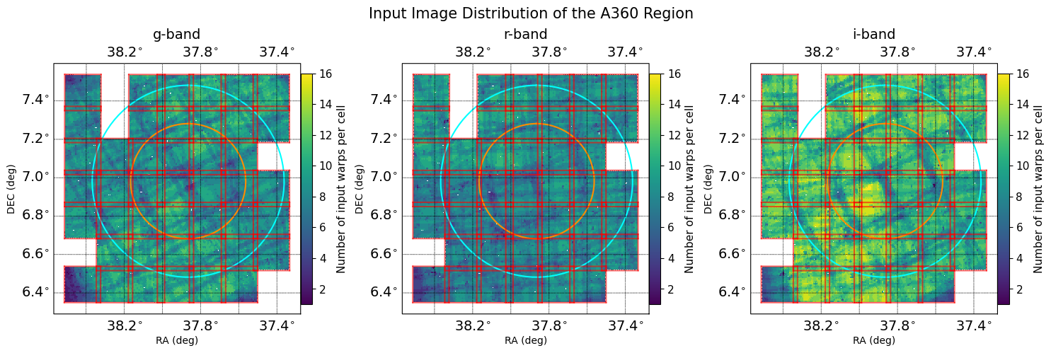
Fig. 1 *These three figures show the input image distribution for the patches, each composed of 484 cells, around A360 in the g, r, and i-bands. The red squares outline the inner patch boundaries, where the 2 cell overlap is visible. The three missing patches are due to processing errors when running Metadetection, though they do not significantly overlap with the 0.5 degree radius around the BCG (cyan circle). Additionally, the 0.3 degree radius (orange circle) contains no missing patches; this radius contains the upper limit of the data used for the final shear profile. The colorbar is scaled to the minimum and maximum number of inputs images across the three bands (1 and 16, respectively). *```#
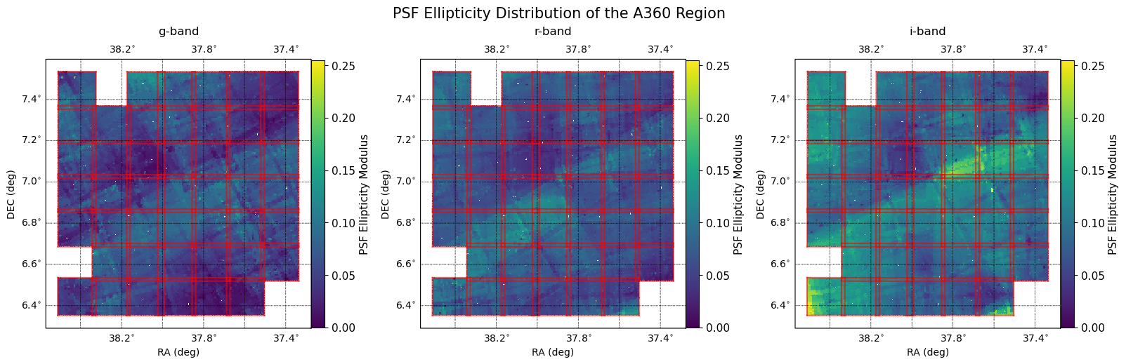
Fig. 2 PSF ellipticity modulus distribution with one PSF realization per cell for the patches around A360 in the g, r, and i-bands. The red squares outline the inner patch boundaries. The i-band plot is in good agreement with a similar plot in [Combet et al., 2025]. The mean ellipticities are 0.0558, 0.0690, and 0.0980 for the g, r, and i-bands, respectively. The colorbar is scaled from 0 to the highest value across the 3 bands, which is about 0.255.#
Note that for cell-based coadds, there is a single PSF model for each cell, realized at the center of the cell. The distribution of PSF ellipticities are seen in Fig. 2.
Exact commands used for generating cell-based coadds#
The exact commands used to generate the cell-based coadds become quite long and are collected here for transparency and to avoid cluttering other sections.
The two following pipetask commands were used to initially generate the cell-based coadds. These collections will also contain the psf_matched_warps and artifact masks needed for later commands. The list is tracts is only shown in the first command, though this list is the same for all commands. These commands below were run on the w_2025_17 weekly stack version of the Pipeline, with the exception of a few user branches in ‘drp_tasks’ and ‘cell_coadds’, with both under the branch u/mirarenee/no_ap_corr. The pipeline file used was nearly the same as the one listed above, with the only exceptions being the numberOfNoiseRealizations and num_noise_realizations, which were not yet utilized.
pipetask run -j 4 --register-dataset-types  \
-b /repo/main \
-i LSSTComCam/runs/DRP/DP1/w_2025_17/DM-50530 \
-o u/$USER/ComCam_Cells/a360 \
-p /sdf/group/rubin/user/mgorsuch/ComCam/pipeline.yaml \
-d "((tract=10463 AND patch IN (30..34,40..44,50..54,60..64,70..74,80..84,90..94)) \
OR (tract=10464 AND patch IN (37..39,47..49,57..59,67..69,77..79,87..89,97..99)) \
OR (tract=10704 AND patch IN (0..5)) \
OR (tract=10705 AND patch IN (8, 9))) \
AND (band='i' OR band='r') AND skymap='lsst_cells_v1'"
pipetask run -j 4 --register-dataset-types  \
-b /repo/main \
-i LSSTComCam/runs/DRP/DP1/w_2025_17/DM-50530 \
-o u/$USER/ComCam_Cells/a360_g \
-p /sdf/group/rubin/user/mgorsuch/ComCam/pipeline.yaml \
-d "tract=10463 ... AND (band='g') AND skymap='lsst_cells_v1'"
The direct_warps were then recreated in order to generate noise realizations that go through the warping process. These were again run on the weekly stack w_2025_17 and the u/mirarenee/no_ap_corr branches for the drp_tasks and cell_coadds packages.
pipetask run -j 4 --register-dataset-types  \
-b /repo/main \
-i LSSTComCam/runs/DRP/DP1/w_2025_17/DM-50530,u/$USER/ComCam_Cells/a360,u/$USER/ComCam_Cells/a360_g \
-o u/$USER/ComCam_Cells/a360/corr_noise \
-p /sdf/group/rubin/user/mgorsuch/ComCam/pipeline-warp-cell.yaml \
-d "tract=10463 ... AND (band='i' OR band='r' OR band='g') AND skymap='lsst_cells_v1'"
The pipeline-warp-cell.yaml file used is below:
description: A simple pipeline to test development of cell-based coadds in ComCam. This assumes that there is a collection already available containing the artifact masks created using MakePsfMatchedWarpTask and CompareWarpAssembleCoaddTask.

instrument: lsst.obs.lsst.LsstComCam

tasks:
    makeDirectWarp:
        class: lsst.drp.tasks.make_direct_warp.MakeDirectWarpTask
        config:
            connections.calexp_list: preliminary_visit_image
            connections.visit_summary: visit_summary
            connections.warp: direct_warp
            connections.masked_fraction_warp: direct_warp_masked_fraction
            doWarpMaskedFraction : true
            doPreWarpInterpolation : true
            numberOfNoiseRealizations : 1
    assembleCellCoadd:
        class: lsst.drp.tasks.assemble_cell_coadd.AssembleCellCoaddTask
        config:
            connections.inputWarps: direct_warp
            connections.visitSummaryList: visit_summary
The pipetask command below was used to incorporate the noise realization implementation in the cell-based coadds. The command was run on the w_2025_34 weekly stack version of the Pipeline, with the exception of a few ticket branches in ‘drp_tasks’ and ‘cell_coadds’, with both under the branch tickets/DM-43585.
pipetask run -j 4 --register-dataset-types  \
-b /repo/main \
-i u/$USER/ComCam_Cells/a360/corr_noise \
-o u/$USER/ComCam_Cells/a360/corr_noise_cells \
-p /sdf/group/rubin/user/mgorsuch/ComCam/pipeline-ap.yaml \
-d "tract=10463 ... AND (band='i' OR band='r' OR band='g') AND skymap='lsst_cells_v1'"
The pipeline-ap.yaml used is found below:
description: A simple pipeline to test development of cell-based coadds in ComCam

instrument: lsst.obs.lsst.LsstComCam

tasks:
    assembleCellCoadd:
        class: lsst.drp.tasks.assemble_cell_coadd.AssembleCellCoaddTask
        config:
            connections.inputWarps: direct_warp
            connections.visitSummaryList: visit_summary
            num_noise_realizations : 1
Running Metadetection#
Metadetection ([Huff and Mandelbaum, 2017], [Sheldon and Huff, 2017], [Sheldon et al., 2020], and most recently [Sheldon et al., 2023]) is a shear calibration software focused on an empirical approach of artificially shearing images of galaxies to measure the response calibration matrix R, which is used to measure the response of the measured shape to an applied shear (see Shear Calibration for more details). The calibration is then applied to the unsheared images to calibrate their shear measurements. Metadetection is the sequel software to the original Metacalibration. The primary difference between the two is that while Metacalibration measures the shear response of individual objects for calibration, Metadetection is designed to detect and measure after the applied shear, resulting in 5 catalogs of shear types (non-sheared, in the plus/minus \(g_1\) direction, and in the plus/minus \(g_2\) direction). The main consequence of this is that since detection is shear-dependent, as seen in [Sheldon et al., 2020], the 5 Metadetection catalogs do not have necessarily the same objects, and cannot be matched to each other; shear is instead calibrated using the mean shape values.
Metadetection is currently being integrated into the LSST Science Pipelines as a pipeline task to fully utilize the cell-based coaddition based tasks in the pipeline structure. Since this is a work-in-progress, the packages used here are not finalized.
Detection is done on an inverse variance weighted average coadd of the three individual band coadds. As for measurement, the algorithm used here is gauss, a forward model that jointly fits each object across the three bands, g, r, and i. These measurements are done pre-PSF (i.e. PSF-deconvolved), so that the flux measurements are less sensitive to changes in the PSF between filters. This feature will be useful for the color-based red sequence cuts.
The Metadetection shear catalog for this technote was run on the w_2025_34 weekly stack version of the Pipeline. As for packages, metadetect used the lsst-dev branch, the ‘cell_coadds’ package again used the tickets/DM-43585 branch, and the drp_tasks package used a custom branch u/mirarenee/meta_test. The drp_tasks user branch was needed to add a few minor changes in order to run Metadetection on more recent pipeline stacks.
The pipetask command used to generate the Metadetection catalog is found below:
pipetask run -j 4 --register-dataset-types \
-b /repo/main \
-i refcats,u/mgorsuch/ComCam_Cells/a360/corr_noise_cells \
-o u/$USER/metadetect/a360_3_band/noise \
-p /sdf/group/rubin/user/mgorsuch/notebooks/metadetect/comcam_pipeline.yaml \
-c metadetectionShear:shape_fitter='gauss' \
-d "skymap='lsst_cells_v1'"
The associated comcam_pipeline.yaml file used for defining the tasks is outline below:
description: Pipeline for running metadetection on DP1
instrument: lsst.obs.lsst.LsstComCam

tasks:
    metadetectionShear:
        class: lsst.drp.tasks.metadetection_shear.MetadetectionShearTask
        config:
            required_bands : ["g", "r", "i"]
            connections.ref_cat: the_monster_20250219
            shape_fitter: "gauss"
            python: |
                config.ref_loader.filterMap = {'lsst_'+band: 'monster_ComCam_%s' % (band) for band in 'ugrizy'}
An important note is that, for this analysis, a single noise image is associated for each cell within Metadetection. A noise image is generated for each exposure that is also subjected to the warping process, which is needed to accurately capture correlated noise ([Sheldon and Huff, 2017], [Sheldon et al., 2020]). The noise distribution is randomly pulled from a Gaussian distribution centered at zero with a variance equal to the median variance of the input exposure.
The raw catalog immediately after running Metadetection contains 1398239 objects total. After removing objects flagged by Metadetection (i.e. objects cut due to measurement failures), there are 984169 total objects. Removing duplicates from patch overlap reduce the catalog to 805401 objects, and removing duplicates from individual cell overlaps leaves 443,615 objects. The non-sheared sub-catalog is consistently ~20% of the total catalog.
Red Sequence Galaxy Identification#
Cluster member galaxies of the lensing cluster structure will not have a lensing signal (at least not from the cluster itself). Due to this, these galaxies need to be identified and removed from the lensing sample to avoid diluting the shear signal ([Medezinski et al., 2018]). These lensing galaxies are primarily identified through visual inspection using color-magnitude plots across three different bands in this technote. Other methods, like photometric redshifts, may also be used, though using only three available bands limits this approach. The red sequence (RS) identification here is done prior to other cuts to more easily visually identify the red sequence galaxies.
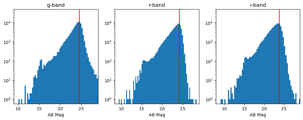
Fig. 3 The distribution of object magnitudes, from Metadetection flux measurements, in each of the bands used. This distribution is after duplicates are removed and Metadetection flagged objects are cut, though prior to red sequence galaxy identification and selection cuts. The red vertical lines indicate the limiting magnitude, determined by eye.#
A series of color-magnitude plots with progressive cuts is used to visually identify the RS galaxies. Each cut is applied to the entire catalog, though only the non-sheared catalog is shown in the color-magnitude plots. Previous visual inspection showed that while there is some variation in-between shear type catalogs, the variation is minimal and random enough that applying the same cuts across all catalogs should be sufficient for this analysis.
The catalog is first cut to galaxies less than 0.1 degree away from the BCG to focus on galaxies that are more likely to be cluster members. The red sequence cluster members are identified in a line of objects with relatively consistent color across a range of magnitudes, with the line being more apparent in the smaller sample of galaxies. This line of galaxies is highlighted with orange points, with the upper and lower limits shown in red. The same visual inspection is done again for the larger sample of galaxies, those within 0.5 degrees of the BCG.
RS galaxies are selected if they satisfy one of the two requirements in all 3 color-magnitude diagrams: the data point falls within the range identified during visual inspection, or the 1-\(\sigma\) error bars for the color measurement intersect the RS range. The error bar requirement is meant to capture potential RS galaxies that may fall out of the selection region due to noisy measurements, particularly at the fainter end. The RS identification is then also limited to galaxies with 18 < gauss_band_mag_r < 24. While RS galaxies may be fainter than this, it becomes more difficult to distinguish between RS and background galaxies. Since unsheared foreground galaxies will dilute the signal, but not bias it, a small contamination is allowed to keep the many source galaxies that may otherwise be cut. Any remaining bright galaxies (those with gauss_band_mag_r < 20) are removed below as described in the selection cut section.
The sample of galaxies within 0.5 degrees of the BCG goes on to further selection cuts in the next section, with the identified RS galaxies removed and masks applied. The masks include bright objects, galactic cirrus, SFD dust, and areas with low numbers of exposures. Mask details can be found in (in prep technote). The impact of cuts applied within the 0.5 degree sample are summarized in Table 2.
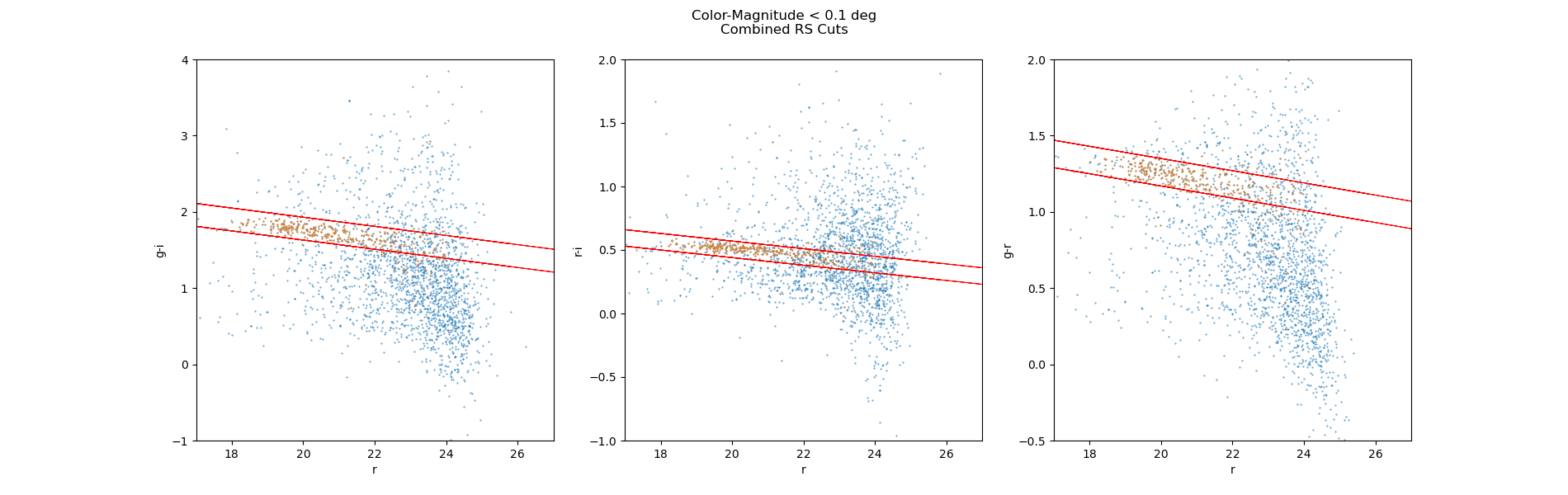
Fig. 4 Color-magnitude diagram cut to 0.1 degrees within the BCG. Objects that are included within the cut are highlighted in orange. Objects included the cut may fall outside of the original red boundary lines if their error bars intersect with the boundaries. Error bars are not shown for clarity.#
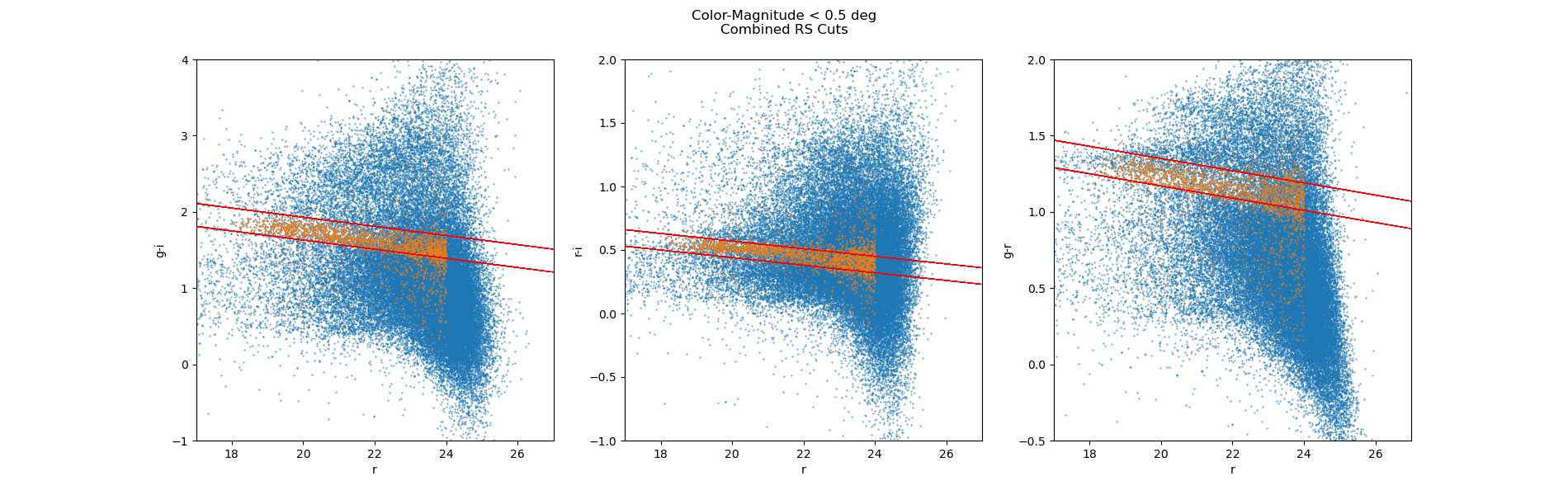
Fig. 5 Color-magnitude diagram cut to 0.5 degrees within the BCG. Objects that are included within the cut are highlighted in orange.#
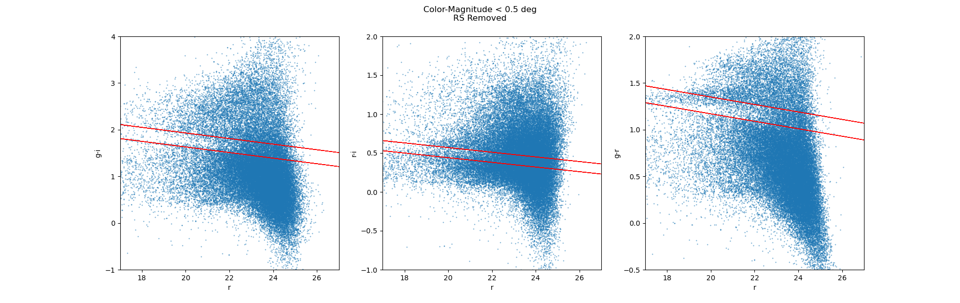
Fig. 6 Color-magnitude diagram cut to 0.5 degrees within the BCG. Objects that are included within the cut are removed.#
Selection Cuts#
Once the RS galaxies are removed and masks are applied, additional selection cuts are introduced. These cuts are primarily based on [Yamamoto et al., 2025], though are customized in several cases to better fit the data from LSSTComCam. A detailed outline of the cuts used and object removed can be seen in Table 1. The Yamamoto cuts describe a size ratio cut, defined as the size of the object squared divided by size of the PSF squared, or \(T^{gauss}/T^{gauss}_{PSF}\). This is used as a star-galaxy cut. For the Yamamoto measurements and the measurements here, these sizes are measured for the pre-PSF objects, so stars will hover around 0 for this ratio. Some notable differences include the magnitude cut, which is based off of Fig. 7, and the junk cuts and size cuts which are specific to DES and don’t seem to appear to affect the final catalog using LSSTComCam data.
Selection Cut |
Rows Removed |
Fraction Removed |
|---|---|---|
|
111442 |
54.4% |
|
30335 |
14.8% |
|
0 |
0.0% |
|
74987 |
36.6% |
|
11161 |
5.5% |
|
355 |
0.2% |
|
49 |
0.02% |
|
574 |
0.3% |
As a visual summary of the cuts done to produce the sample, it’s helpful to plot the distribution of magnitudes, in a similar vein as Figure 2 in [Applegate et al., 2014]. A description of each label can be found in Table 2, along with the numbers in the non-sheared catalog after each cut is applied. Some of the selection cuts are separated into their own rows to better capture their individual impact. Of particular note is the i_mag cut: while [Adari et al., 2025] uses a cut of 24.0, a smaller cut of 23.5 is chosen to reduce the significance of the SNR cut. We don’t want SNR to be a significant cut since the photo-z data used was trained on the Extended Chandra Deep Field South (ECDFS) data, which has different properties in depth than the A360 field.
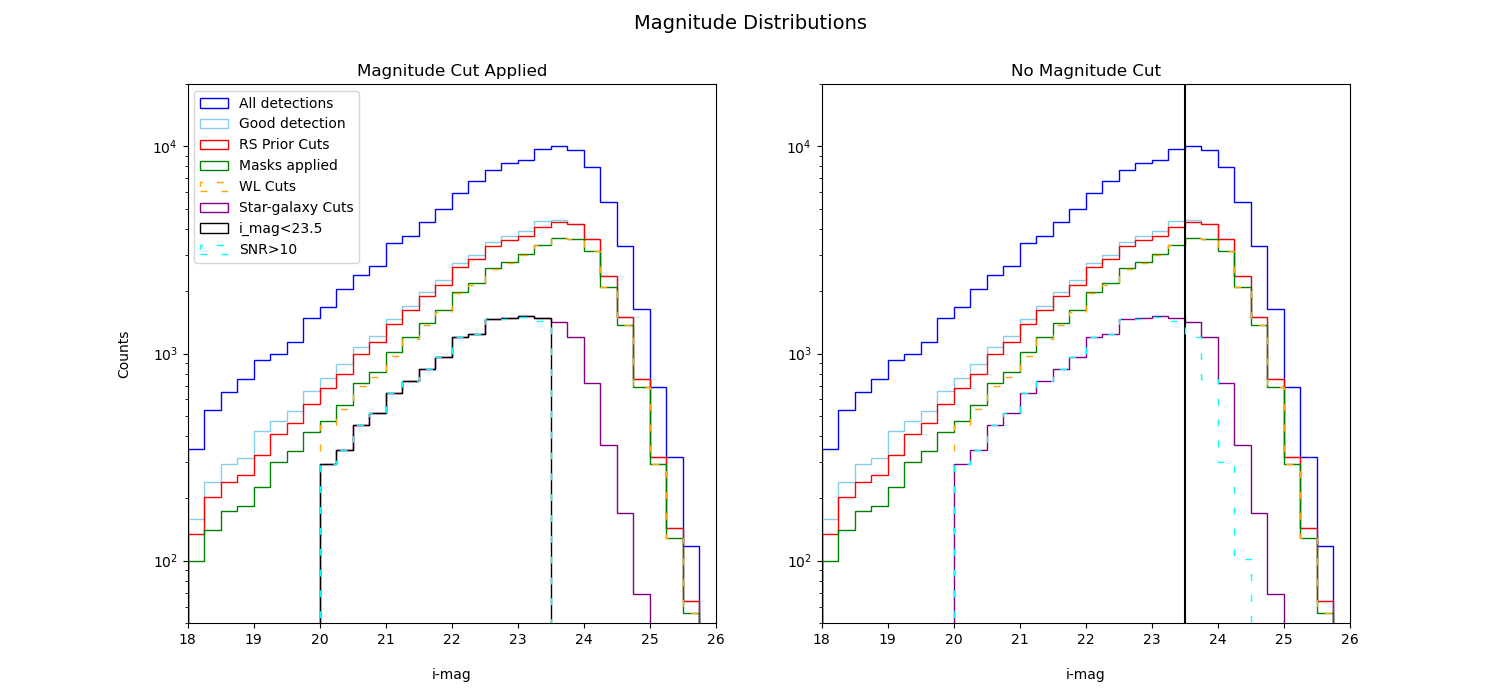
Fig. 7 Magnitude distributions of the i-band after various cuts done to produce the weak lensing sample. Left: All cuts are applied in the order described in Table 2. Right: The magnitude cut is not applied to show where the SNR cut becomes significant at fainter magnitudes and begins to remove a substantial number of objects. The magnitude cut is instead represented by the vertical line.#
Cut Name |
Description |
Rows in non-sheared catalog (% of total catalog) |
|---|---|---|
All detections |
Detections that have a finite i-band magnitude |
172157 (20.022%) |
Good detections |
Flagged and duplicate objects removed |
54228 (20.006%) |
RS Cuts |
Red sequence galaxies are identified and removed |
51804 (20.009%) |
Masks |
Masks are applied |
40949 (20.000%) |
WL Cuts |
Selection cuts |
38297 (19.999%) |
Star-galaxy |
Size ratio cut to remove stars from the sample |
17171 (19.993%) |
Magnitude Cut |
Magnitude where SNR begins to remove objects |
13190 (19.998%) |
SNR Cut |
Objects with SNR < 10 are removed |
13114 (19.989%) |
For reference against another catalog, it’s useful to look at the number of objects found in the HSM catalog ([Hirata and Seljak, 2003], [Mandelbaum et al., 2006]) used in [Combet et al., 2025] within the same 0.5 degree radius as used in this technote. The HSM catalog first reads in 175383 objects prior to any cuts, and then 12852 objects after all cuts are applied. This is a similar ballpark as the final Metadetect catalog size of 13114, especially considering that the selection and quality cuts of two catalogs differ due to the nature of separate catalogs.
The source density across all radial bins for Metadetection is 6.1 \(\pm\) 0.09 \(\text{arcmin}^{-2}\), with the density across individual bins shown in Fig. 8. The density for the Metadetection catalog does trend lower than the HSM catalog, which has a range of 7-8 \(\text{arcmin}^{-2}\). This is most likely due to the final sizes of the different catalogs, though it should also be noted that the HSM catalog does not yet incorporate masks, which will affect both the final number count and effective area covered by the catalog.
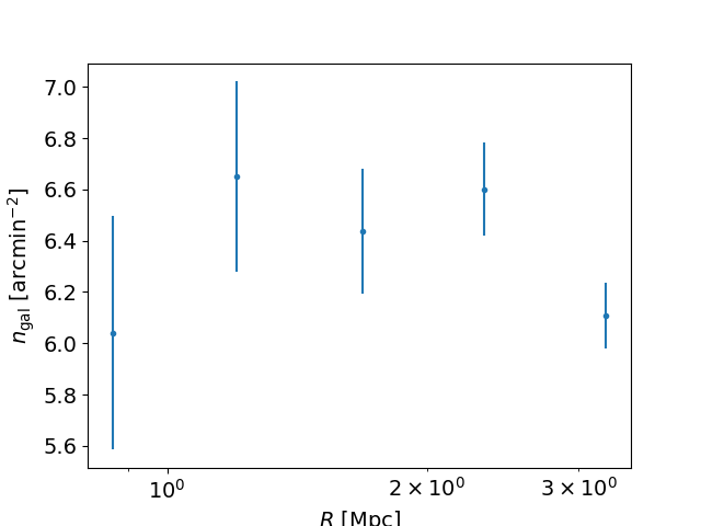
Fig. 8 The galaxy density within each radial bin used for the shear profile. Error bars are one standard deviation Poisson shot noise. Area that has been masked is removed from the calculation.#
Photo-Z Data#
In order to model a shear profile to compare to the observed data, an \(N(z)\) estimate will be needed. With the utilities available in the Cluster Lensing Mass Modeling (CLMM) code [Aguena et al., 2021], there is a default source redshift distribution based off of the DESC Science Requirements Document (SRD, [The LSST Dark Energy Science Collaboration et al., 2018]) Y10 N(z). However, this is not very representative of the data that’s being used here, which is comparatively much shallower. Instead, the initial photo-z catalog used here is created with DNF ([De Vicente et al., 2016]) on DP1 data, produced in the same manner as described in [Adari et al., 2025].
The objects in the Metadetection catalogs are then matched to the objects in the DP1 catalogs by nearest neighbor, based on RA/DEC coordinates and limited to matches within 1 arcsecond. The matching is only needed for the non-sheared catalog, which is the catalog used for the \(N(z)\) estimate. Objects are then additionally cut from the matched catalogs if they fall below a redshift estimate of 0.37, based on the cut used in [Adari et al., 2025]. The final number in the matched photo-z catalog is 9328 for the non-sheared subset. The \(N(z)\) generated by the method above is not used for the shear profile generated by the data, only for the test model used for reference. Future works with Metadetection data should run photo-z algorithms on each of the shear profile catalogs individually to fully capture the additional selection effects within the response.
Once the matched catalogs are created, and using a standard cosmology (\(\Omega_m=0.3\), \(h=0.7\)), the statistics of the lensing efficiency can be calculated. The CLMM package has tools for calculating these using the photo-z point estimate of each galaxy, with the theory based on [Schrabback et al., 2018], which will be summarized below.
First off is the geometric lensing efficiency \(\beta\), which is the ratio between \(D_{ls}\) and \(D_s\), the angular diameter distances between the lens and and the source, and the observer to the source, respectively. \(\beta\) is not allowed to go below zero, as sources in front cluster will have no contribution to the lensing signal. The \(\beta_s\) term then is the ratio of \(\beta\)’s of a source at a specific redshift, and a test source at infinite redshift (set to \(z=1000\) by default).
From the matched source galaxy sample, the statistics of these \(\beta\) parameters can be calculated. Weights can be implemented, though this analysis simply sets the weights to 1 to produce a simple mean.
With the mean \(\beta_s\) statistics a curve predicting the shape of the reduced shear as a function of \(R\), the projected radial distance from the BCG in Mpc, is approximately given by
The terms \(\gamma_{\infty}\) and \(\kappa_{\infty}\) represent the shear and convergence of a test source at infinite redshift, with the \(\left<\beta_s\right>\) and \(\left<\beta_s^2\right>\) terms modulating the theoretical reduced shear based on the ensemble redshift information from the matched source catalog.
Shear Calibration#
Understanding the relationship between the shear applied to an object and the effect of that shear on measuring the object’s shape is a critical step to calibrating the catalog’s shear measurements. The main purpose of Metadetection’s 5 sub-catalogs is to calculate the linear response matrix, R.
The main assumption is that the weak lensing shear signal is small enough that we can Taylor expand the measured galaxy ellipticity about a zero shear signal. The first term goes to 0 in the limit of a large enough sample of galaxies where the shape noise averages out. The relation between the measured galaxy ellipticity and the resulting shear signal is controlled by R, the linear response of the ellipticity to an applied shear. Within the Metadetection framework, the components of R can be calculated by taking the mean measured galaxy ellipticities of the 4 artificially shear object catalogs. The magnitude of the applied shear in each catalog is 0.01, to make \(\Delta\gamma_j\) a total of 0.02 for each component of R. Once R is calculated, it’s applied to the mean non-sheared object ellipticities to produce the calibrated reduced shear.
In the specific case of cluster lensing, we are more interested in the tangential and cross shears around the cluster, split into radial bins. The response matrix R is first calculated on all galaxy ellipticities measurements from the four sheared catalogs, after all applied cuts, but prior to binning in order to improve the uncertainty of R. The calibration is then applied to the galaxies in the non-sheared catalog, producing the reduced shear. Using the utilities in CLMM, the mean tangential and cross terms are calculated from the calibrated shears for each radial bin.
A note on coordinate systems: Both the Metadetection \(g_1\) and \(g_2\) shapes and the CLMM code used here utilize the “Euclidean” definition described in section 5.1 of [Rowe et al., 2015].
Shear Results#
The resulting shear profile is shown below in Fig. 9. Each bin is calculated from the calibrated shapes of galaxies in five bins that range from 0.71 Mpc to 3.75 Mpc, split evenly in \(\log_{10}\) space. The range for the binning is based off of [Grandis et al., 2021]. The error bars for the bins are 1 standard error (standard deviation / \(\sqrt(N)\)). From smallest radial separation to largest, the number of galaxies in each bin are 175, 320, 691, 1326, and 2216 galaxies. Despite shear around clusters typically being fairly noisy, there is a visible upward trend in the tangential shear, with the cross shear typically hovering around 0.
The Mpc distances are assuming a cluster redshift of z=0.22 ([Quintana and Ramirez, 1995]).
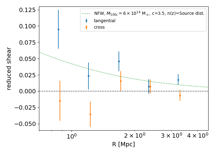
Fig. 9 The reduced shear profile around A360 for both tangential and cross shear measurements, using the cuts described throughout the technote. The dotted green line represents a reference NFW model. Error bars are 1 standard error. Detection significance for the tangential and cross shears are 3.70 and 0.39 sigma, respectively.#
The theoretical shear profile is produced using CLMM. This profile is purely for a rough reference, and is not fit to the calibrated shear data. The profile is using an NFW halo with an estimated cluster mass of 6e14 solar masses ([Hilton et al., 2021]) and a concentration of 3.5. The source redshift distribution is based off of the mean \(\beta_s\) statistics described in the photo-z section above.
Galaxies < 0.5 degrees |
|
|---|---|
R_11 |
0.6785 |
R_22 |
0.6737 |
R_11_err |
0.00330 |
R_22_err |
0.00333 |
| R_11 - R_22 | |
0.0048 |
Validation & Testing#
This section contains a non-exhaustive list of notes and figures on characterizing the Metadetection output catalog and the effects from various cuts.
Object Size and S/N Cuts#
The measured object size compared to the signal-to-noise ratio is a simple cut to differentiate stars and galaxies.
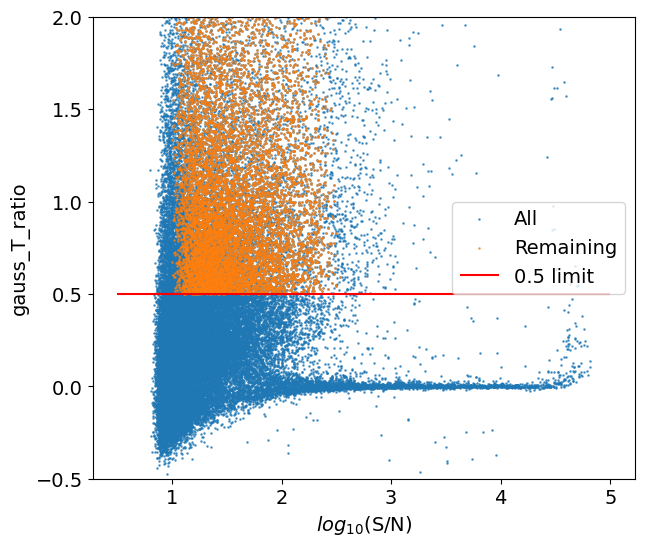
Fig. 10 The relationship between the object size ratio and the S/N of each object before and after selection cuts (both with red sequence galaxies removed). The red line is a visual reference to see what objects are removed by the 0.5 object size ratio cut, though other objects may be removed due to additional cuts. Stars are expected to fall near an object ratio of 0, which is seen clearly for high S/N objects in blue. The remaining objects in orange have the line of stars removed, though some low S/N stars may survive the cut, as those tend to have higher size uncertainties as seen in [Yamamoto et al., 2025]. The spurious, high S/N objects that appear in blue are primarily removed with the applied bright object and galactic cirrus masks from (in prep technote).#
Object Distributions#
Plotting the distribution of objects on the sky is a simple but effective way to discover inconsistencies within the data. For example, the leftmost plot in Fig. 11 shows an overdensity of objects detected that aligns with where patches overlap, unexpected after removing exact duplicates based on RA and DEC coordinates. This duplication is addressed, as seen in the middle and right-most plots in Fig. 11.
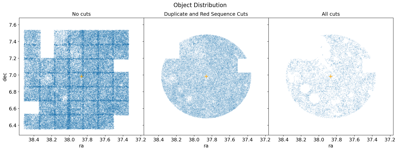
Fig. 11 Object distributions of the non-sheared catalog at various points during cuts. Left: Galaxy distributions prior to any cuts. There is a clear overdensity that overlaps between patches. Middle: the distribution after the duplicates and red sequence galaxies have been removed. Right: the object distribution after all cuts have been applied.#
Final Remarks#
From what was able to be achieved within this technote, the combination of cell-based coadds and Metadetection have the necessary infrastructure needed to successfully run end-to end within the LSST Science Pipelines ecosystem and produce a shape catalog. With this shape catalog, a tangential shear profile of A360 is detected. This is a significant technical milestone, especially considering that the data for this field is shallow and has limited band information. Some future validation work could include testing alternative blending algorithms to potentially improve the performance of shear measurements in crowded cluster environments, obtaining PSF measurements for reserved stars to preform a \(\rho\)-statistics analysis, and SSI analyses such as completion tests. Running Metadetection on additional DP1 fields may also identify edge-cases that were not uncovered within the A360 field.
At this time, the task for running Metadetection is still under development, particularly needing focus in robustness and computing efficiency. It should be noted that many configuration settings are not yet available to the pipeline infrastructure through pipeline .yaml files. The main motivation for custom branches was to enable these changes (e.g. changing wmom to gauss) for testing purposes within this specific use case.
Acknowledgement: We thank Erin Sheldon for his guidance and clarification on Metadetection details and associated outputs. Several details within the technote directly benefit from this improved clarity.
References#
Prakruth Adari, Anja von der Linden, Tianqing Zhang, and others. Source Selection for Abell 360 in LSSTComCam Data Preview 1. Commissioning Technical Note SITCOMTN-163, NSF-DOE Vera C. Rubin Observatory, July 2025. URL: https://sitcomtn-163.lsst.io/, doi:10.71929/rubin/2571157.
C. Combet, A. Plazas Malagón, S. Fu, and others. PSF assessment in the field of Abell 360 and shapeHSM shear profile using LSSTComCam data. Commissioning Technical Note SITCOMTN-161, NSF-DOE Vera C. Rubin Observatory, November 2025. URL: https://sitcomtn-161.lsst.io/, doi:10.71929/rubin/2572986.
Arun Kannawadi and James Bosch. Producing weak lensing shear catalogs from LSST Science Pipelines. Project & Community Workshop 2023, Tucson, AZ, USA., July 2023. URL: https://project.lsst.org/meetings/rubin2023/agenda/producing-weak-lensing-shear-catalogs-lsst-science-pipelines.
Xiangchong Li, Prakruth Adari, Anja von der Linden, and Rachel Mandelbaum. AnaCal Shear Profile of Abell 360 in LSSTComCam Data Preview 1. Commissioning Technical Note SITCOMTN-164, NSF-DOE Vera C. Rubin Observatory, November 2025. URL: https://sitcomtn-164.lsst.io/, doi:10.71929/rubin/3000577.
M. Yamamoto, M. R. Becker, E. Sheldon, and others. Dark energy survey year 6 results: cell-based coadds and metadetection weak lensing shape catalogue. 2025. URL: https://arxiv.org/abs/2501.05665, arXiv:2501.05665, doi:10.1093/mnras/staf1661.
Conghao Zhou, Tesla Jeltema, Anja von der Linden, and others. Surface brightness profiles around massive galaxies in LSSTComCam data. Commissioning Technical Note SITCOMTN-165, NSF-DOE Vera C. Rubin Observatory, November 2025. URL: https://sitcomtn-165.lsst.io/, doi:10.71929/rubin/3000576.
M. Aguena, C. Avestruz, C. Combet, and others. CLMM: a LSST-DESC cluster weak lensing mass modeling library for cosmology. MNRAS, 508(4):6092–6110, December 2021. arXiv:2107.10857, doi:10.1093/mnras/stab2764.
Douglas E. Applegate, Anja von der Linden, Patrick L. Kelly, and others. Weighing the Giants - III. Methods and measurements of accurate galaxy cluster weak-lensing masses. MNRAS, 439(1):48–72, March 2014. arXiv:1208.0605, doi:10.1093/mnras/stt2129.
Robert Armstrong, Erin Sheldon, Eric Huff, and others. The little coadd that could: Estimating shear from coadded images. arXiv e-prints, pages arXiv:2407.01771, July 2024. arXiv:2407.01771, doi:10.48550/arXiv.2407.01771.
J. De Vicente, E. Sánchez, and I. Sevilla-Noarbe. DNF - Galaxy photometric redshift by Directional Neighbourhood Fitting. MNRAS, 459(3):3078–3088, July 2016. arXiv:1511.07623, doi:10.1093/mnras/stw857.
Sebastian Grandis, Sebastian Bocquet, Joseph J. Mohr, Matthias Klein, and Klaus Dolag. Calibration of bias and scatter involved in cluster mass measurements using optical weak gravitational lensing. MNRAS, 507(4):5671–5689, November 2021. arXiv:2103.16212, doi:10.1093/mnras/stab2414.
M. Hilton, C. Sifón, S. Naess, and others. The Atacama Cosmology Telescope: A Catalog of >4000 Sunyaev-Zel\textquoteright dovich Galaxy Clusters. ApJS, 253(1):3, March 2021. arXiv:2009.11043, doi:10.3847/1538-4365/abd023.
Christopher Hirata and Uroš Seljak. Shear calibration biases in weak-lensing surveys. MNRAS, 343(2):459–480, August 2003. arXiv:astro-ph/0301054, doi:10.1046/j.1365-8711.2003.06683.x.
Eric Huff and Rachel Mandelbaum. Metacalibration: Direct Self-Calibration of Biases in Shear Measurement. arXiv e-prints, pages arXiv:1702.02600, February 2017. arXiv:1702.02600, doi:10.48550/arXiv.1702.02600.
Xiangchong Li, Rachel Mandelbaum, Mike Jarvis, Yin Li, Andy Park, and Tianqing Zhang. A differentiable perturbation-based weak lensing shear estimator. MNRAS, 527(4):10388–10396, February 2024. arXiv:2309.06506, doi:10.1093/mnras/stad3895.
Rachel Mandelbaum, Christopher M. Hirata, Mustapha Ishak, Uroš Seljak, and Jonathan Brinkmann. Detection of large-scale intrinsic ellipticity-density correlation from the Sloan Digital Sky Survey and implications for weak lensing surveys. MNRAS, 367(2):611–626, April 2006. arXiv:astro-ph/0509026, doi:10.1111/j.1365-2966.2005.09946.x.
Elinor Medezinski, Masamune Oguri, Atsushi J. Nishizawa, and others. Source selection for cluster weak lensing measurements in the Hyper Suprime-Cam survey. PASJ, 70(2):30, March 2018. arXiv:1706.00427, doi:10.1093/pasj/psy009.
NSF-DOE Vera C. Rubin Observatory. Legacy Survey of Space and Time Data Preview 1 [Data set]. 2025. URL: https://www.osti.gov//servlets/purl/2570308, doi:10.71929/RUBIN/2570308.
H. Quintana and A. Ramirez. Redshifts of 165 Abell and Southern Rich Clusters of Galaxies. ApJS, 96:343, February 1995. doi:10.1086/192122.
B. T. P. Rowe, M. Jarvis, R. Mandelbaum, and others. GALSIM: The modular galaxy image simulation toolkit. Astronomy and Computing, 10:121–150, April 2015. arXiv:1407.7676, doi:10.1016/j.ascom.2015.02.002.
Rubin Observatory Science Pipelines Developers. The LSST Science Pipelines Software: Optical Survey Pipeline Reduction and Analysis Environment. Project Science Technical Note PSTN-019, NSF-DOE Vera C. Rubin Observatory, December 2025. URL: https://pstn-019.lsst.io/, doi:10.71929/rubin/2570545.
T. Schrabback, D. Applegate, J. P. Dietrich, and others. Cluster mass calibration at high redshift: HST weak lensing analysis of 13 distant galaxy clusters from the South Pole Telescope Sunyaev-Zel'dovich Survey. MNRAS, 474(2):2635–2678, February 2018. arXiv:1611.03866, doi:10.1093/mnras/stx2666.
Erin S. Sheldon, Matthew R. Becker, Michael Jarvis, Robert Armstrong, and LSST Dark Energy Science Collaboration. Metadetection Weak Lensing for the Vera C. Rubin Observatory. The Open Journal of Astrophysics, 6:17, May 2023. arXiv:2303.03947, doi:10.21105/astro.2303.03947.
Erin S. Sheldon, Matthew R. Becker, Niall MacCrann, and Michael Jarvis. Mitigating Shear-dependent Object Detection Biases with Metacalibration. ApJ, 902(2):138, October 2020. arXiv:1911.02505, doi:10.3847/1538-4357/abb595.
Erin S. Sheldon and Eric M. Huff. Practical Weak-lensing Shear Measurement with Metacalibration. ApJ, 841(1):24, May 2017. arXiv:1702.02601, doi:10.3847/1538-4357/aa704b.
SLAC National Accelerator Laboratory and NSF-DOE Vera C. Rubin Observatory. Lsst commissioning camera. 2024. URL: https://www.osti.gov//servlets/purl/2561361, doi:10.71929/RUBIN/2561361.
The LSST Dark Energy Science Collaboration, Rachel Mandelbaum, Tim Eifler, and others. The LSST Dark Energy Science Collaboration (DESC) Science Requirements Document. arXiv e-prints, pages arXiv:1809.01669, September 2018. arXiv:1809.01669, doi:10.48550/arXiv.1809.01669.
Vera C. Rubin Observatory Team. The Vera C. Rubin Observatory Data Preview 1. Technical Note RTN-095, NSF-DOE Vera C. Rubin Observatory, September 2025. URL: https://rtn-095.lsst.io/, doi:10.71929/rubin/2570536.
Vera C. Rubin Observatory. An Interim Report on the LSSTComCam On-Sky Campaign. Commissioning Technical Note SITCOMTN-149, NSF-DOE Vera C. Rubin Observatory, August 2025. URL: https://sitcomtn-149.lsst.io/, doi:10.71929/rubin/2574402.